With Google BigQuery ML you can now predict your Google Cloud spend in just a few minutes and without leaving your BigQuery Console UI.

Introduction

Linear Regression, although very simple, can be used to generate accurate predictions for various real world problems efficiently. Due to its simplicity, linear regression training is easy to configure and benefits from fast convergence.

In this post, I will explain how to analyze Google Cloud billing data and build a simple prediction model to estimate the expected overall monthly expenditure. To make it more interesting, I will use only Google BigQuery, thereby keeping all the billing data in the data warehouse ecosystem.

In this exercise, I am going to use Google Billing Exports. Billing export to BigQuery enables customers to export daily usage and charges automatically throughout the day to a BigQuery dataset you specify. You can read about Google Billing Exports here.

The data and code samples are available here: https://github.com/doitintl/BigQueryML-Examples

Raw Data

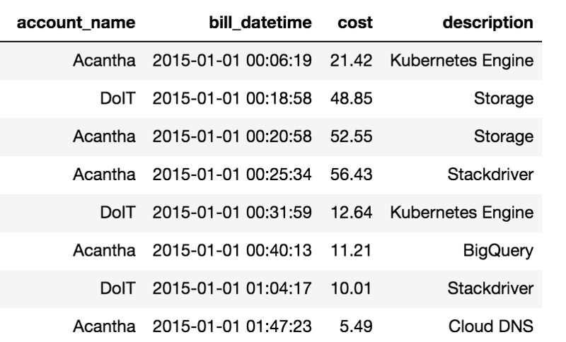
The table below lists the billings for various services consumed by two Google Cloud billing accounts we own.

Desired Model

The goal is to estimate the current month’s total bill based on all the billings received until a given day.

The model will enable the client to not only estimate overall expenditure, but will also detect anomalies and create alerts for overcharges.

Assumptions

The model assumes that the monthly bill is linearly dependant on 3 variables:

The first variable represents the current daily consumption trend. The other two variables are the number of days until the end of the month and the current balance. Together, the model can use these variables to estimate the remaining monthly expenditure.

Data Preparation

Aggregating the data at Daily Resolution

Since the model requires data at the daily resolution, we will use BigQuery to aggregate the data by day.

The resulting scheme looks like this:

account_name — the account id
day — remaining days to the end of the month
month — billing month
year — billing year
daily_cost — the total cost paid for all services during the billing day
monthly_cost — the label, which is the sum all billings made during current month, including future billing

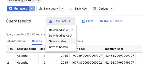
Now that the data is aggregated at daily resolution, I save it as a new table and use it to generate an ML dataset.

Calculating Window Aggregations

The next step is to calculate how much has been billed to each account from the beginning of the month until the current day. We will use an aggregate window function to do this. This function will also enable us to calculate the month’s average daily spending, until the current day.

The syntax for the aggregate window function can be found here: [1]

analytic_function_name ( [ argument_list ] )
  OVER (
    [ PARTITION BY partition_expression_list ]
    [ ORDER BY expression [{ ASC | DESC }] [, ...] ]
    [ window_frame_clause ]
  )

I use the function on our billing_daily_monthly table as follows:

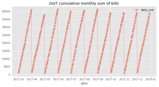
Plotting the data shows that the monthly bill compounds in a somewhat linear manner:

The results above give us confidence that a linear model is an appropriate choice for the expenditure problem. In addition, the gradient has little variance between months, which suggests that the selected features are sufficient statistics with reference to the independent variable.

Obviously, more features and more complex models will likely produce more accurate predictions — those can be built with other tools like Google Cloud ML. But for now it looks like we are done preparing the data.

(WOO HOO!)

Fitting a Linear Regression model using BigQuery ML

Once the data are ready, I can use the new (as of August 2018) BigQuery ML tool to fit a Linear Regression model to the data.

Fitting the model to our dataset is insanely simple !

Making Predictions and Evaluating the Model

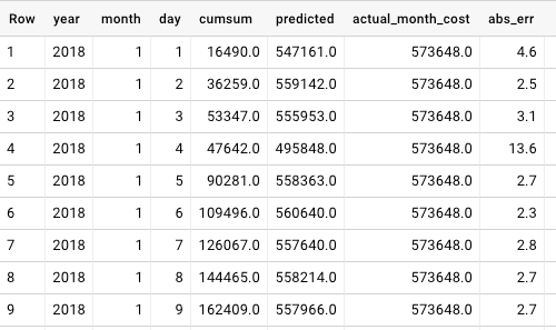
Once saved, the model can be used to make predictions. To do so, I use the following query, which both estimates the final monthly expenditure and calculates the Relative Absolute Error of the predictions per day:

The results demonstrated in the following table can now be saved and serve other components of the system including monitoring and alerting applications. The model’s Mean Relative Absolute Error is approximately 3.0%, which isn’t bad. (Note, the data were generated especially for this demo. With real data, I achieved around 2.0% error)

Want more stories? Check our blog, or follow Gad on Twitter.

Acknowledgments:
Vadim Solovey — Editing
amiel m — Technical Review

Keywords: BigQueryML, BigQuery ML tutorial, BigQuery ML example